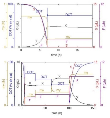
X: Bomass concentration; S: Limiting substrate concentration; DOT: Dissolved oxygen tension;
my: Specific growth rate;  F: Medium flow rate

This simulation illustrates how to start and control a chemostat. The process variables are here plotted against time, while the simulation with chemostat_ss shows the variables plotted against dilution rate (D)

Upper graph: The 10 L process was started as a batch with 15 g/L limiting S. When this substrate was consumed after about 7 hrs (seen from the rapid increase in DOT) the chemostat process was started with a medium containing Si=15 g/L and with the flow rate F=2 L/h, which gives D=0.2 h^-1.

The time scale of the simulation was automatically changed to 0-150 hrs at time 19 hrs without interruption of simulation.

Lower panel: At 30 hrs F was increased to 3 L/h. Check the effects on the state variables! At 64 hrs Si was increased from 15 to 20 g/L. Check the effects on the state variables! At 100 hrs the flow rate F was increased to 8 L/h. What happened and why?

Note that the model can not handle oxygen limitation. The model assumes obligately aerobic metabolism.